Literate Blogging

Literate programming is a methodology that combines a programming language with a documentation language, thereby making programs more robust, more portable, more easily maintained, and arguably more fun to write than programs that are written only in a high-level language. The main idea is to treat a program as a piece of literature, addressed to human beings rather than to a computer. The program is also viewed as a hypertext document, rather like the World Wide Web.

Literate Programming by Donald Knuth (1983) is a seminal book that introduces the concept of literate programming. Using technology available in 2014 we can make a small but important change to the last sentence:

The program is also viewed as a hypertext document on the World Wide Web.

This blog post is an example for such a document. The page is written in markdown (markdown file available here), and all embedded code was executed when this page was generated, i.e. when the markdown was converted to HTML and the blog post was published. To demonstrate this I have embedded code in three different languages below - the output is the second code block.

In R you have

cat('Hello, R world!\n')

Hello, R world!

Or Python

print "Hello, Python world!"

Hello, Python world!

Or Ruby

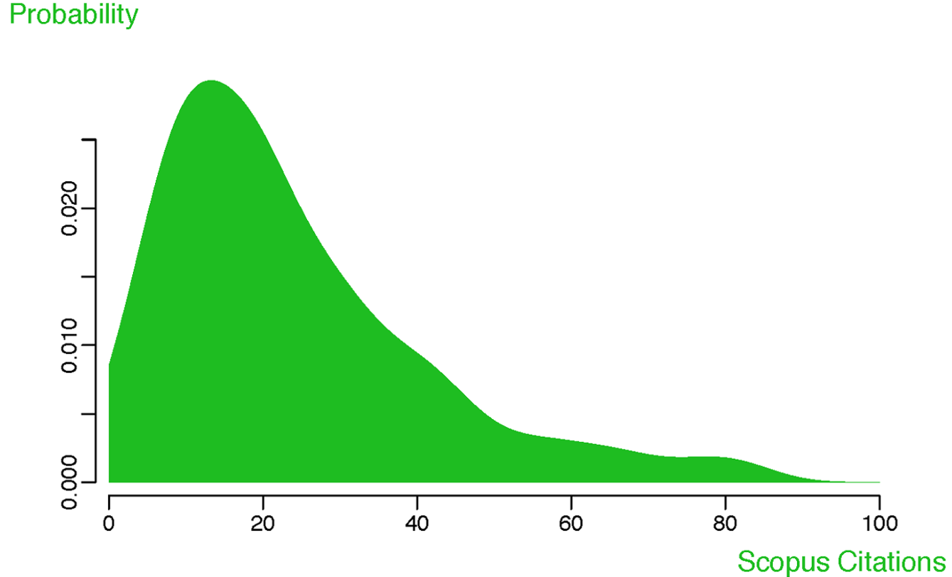
puts 'Hello, Ruby world!'

Hello, Ruby world!

You can also embed code within text blocks (inline), so that 3.48 * 723 becomes 2516.04. Another important option is to generate figures using the embedded code, e.g. the following figure taken from a recent publication.

# code for figure 1: density plots for citation counts for PLOS Biology
# articles published in 2010

# load May 20, 2013 ALM report
alm <- read.csv("data/alm_report_plos_biology_2013-05-20.csv", stringsAsFactors = FALSE)

# only look at research articles
alm <- subset(alm, alm$article_type == "Research Article")

# only look at papers published in 2010
alm$publication_date <- as.Date(alm$publication_date)
alm <- subset(alm, alm$publication_date > "2010-01-01" & alm$publication_date <=
    "2010-12-31")

# labels
colnames <- dimnames(alm)[[2]]
plos.color <- "#1ebd21"
plos.source <- "scopus"

plos.xlab <- "Scopus Citations"
plos.ylab <- "Probability"

quantile <- quantile(alm[, plos.source], c(0.1, 0.5, 0.9), na.rm = TRUE)

# plot the chart
opar <- par(mai = c(0.5, 0.75, 0.5, 0.5), omi = c(0.25, 0.1, 0.25, 0.1), mgp = c(3,
    0.5, 0.5), fg = "black", cex.main = 2, cex.lab = 1.5, col = plos.color,
    col.main = plos.color, col.lab = plos.color, xaxs = "i", yaxs = "i")

d <- density(alm[, plos.source], from = 0, to = 100)
d$x <- append(d$x, 0)
d$y <- append(d$y, 0)
plot(d, type = "n", main = NA, xlab = NA, ylab = NA, xlim = c(0, 100), frame.plot = FALSE)
polygon(d, col = plos.color, border = NA)
mtext(plos.xlab, side = 1, col = plos.color, cex = 1.25, outer = TRUE, adj = 1,
    at = 1)
mtext(plos.ylab, side = 2, col = plos.color, cex = 1.25, outer = TRUE, adj = 0,
    at = 1, las = 1)

par(opar)

All this functionality is provided by knitr, a package for the R statistical programming language. knitr has been around for a while, but integration into the Jekyll blogging platform is still fragile. Earlier this week at the rOpenSci hackathon (more on this later) a group of us worked hard to improve this integration. We are still not completely done, but the source code is available here. Most importantly, all the conversion happens on the server, and we are only using freely available tools. I have now enabled this functionality for this blog, so expect more code embedded examples in the future.

References

Fenner, M. (2013). What can article-level metrics do for you? PLoS Biol, 11(10), e1001687. doi:10.1371/journal.pbio.1001687

Knuth, D. E., Stanford University, & Computer Science Department. (1983). Literate programming. Stanford, CA: Dept. of Computer Science, Stanford University.